vtune的安装和profile
使用
由于snode0有sudo
1 | source /opt/intel/oneapi/setvars.sh |
sudo后图形化界面 MobaXterm打不开的原因参考这个
Step1 : Performance Snapshot 参数说明
以IPCC2022 初赛 支撑点计算的baseline为例
Logical Core Utilization
1 | Effective Logical Core Utilization: 3.8% (2.436 out of 64) |
CPU利用率主要是指计算有效占比。为100%意味着所有逻辑CPU都是由应用程序的计算占用。
Microarchitecture Usage
微架构使用指标是一个关键指标,可以帮助评估(以%为单位)你的代码在当前微架构上运行的效率。
微架构的使用可能会受到
- long-latency memory长延迟访存、
- floating-point, or SIMD operations浮点或SIMD操作的影响;
- non-retired instructions due to branch mispredictions;由于分支错误预测导致的未退役指令;
- instruction starvation in the front-end.前端指令不足。
vtune的建议
1 | Microarchitecture Usage: 37.7% of Pipeline Slots |
针对Back-End Bound: 23.8%的建议如下:
A significant portion of pipeline slots are remaining empty.
(??? 他是指有23.8% empty还是被使用了呢)
When operations take too long in the back-end, they introduce bubbles in the pipeline that ultimately cause fewer pipeline slots containing useful work to be retired per cycle than the machine is capable to support.
This opportunity cost results in slower execution.
- Long-latency operations like divides and memory operations can cause this,
- as can too many operations being directed to a single execution port (for example, more multiply operations arriving in the back-end per cycle than the execution unit can support).
针对Bad Speculation: 21.5%的建议如下:
A significant proportion of pipeline slots containing 21.5% useful work are being cancelled.
This can be caused by mispredicting branches or by machine clears. Note that this metric value may be highlighted due to Branch Resteers issue.
Retiring metric
Retiring metric represents a Pipeline Slots fraction utilized by useful work, meaning the issued uOps that eventually get retired.
Retiring metric 表示有用工作所使用的Pipeline slot流水线管道的比例,所有发射的uOps最终都会retired。
Ideally, all Pipeline Slots would be attributed to the Retiring category.
理想情况下,所有的管道槽都应该归于退休类别。
Retiring of 100% would indicate the maximum possible number of uOps retired per cycle has been achieved. 100%的退役表明每个周期内退役的uop数量达到了可能的最大值。
Maximizing Retiring typically increases the Instruction-Per-Cycle metric.
最大化Retiring通常会增加IPC。
Note that a high Retiring value does not necessary mean no more room for performance improvement.
For example, Microcode assists are categorized under Retiring. They hurt performance and can often be avoided.
Microcode assists根据Intel的解释是
当遇到特殊的计算(比如处理非常小的浮点值(所谓的逆法线)时),浮点单元并没有被设置为本机执行这些操作。为此需要在指令流中插入可能有数百个指令长的小程序,对性能会造成很大的影响。
Front-End Bound
Front-End Bound metric represents a slots fraction where the processor’s Front-End undersupplies its Back-End. 该指标表示前端产生的指令是否足以支持后端处理。
Front-End denotes the first part of the processor core responsible for fetching operations that are executed later on by the Back-End part. 前端将指令分解成uops供后端处理。
Within the Front-End, a branch predictor predicts the next address to fetch, cache-lines are fetched from the memory subsystem, parsed into instructions, and lastly decoded into micro-ops (uOps). 在前端中,分支预测器预测下一个要获取的地址,缓存行从内存子系统中获取,解析为指令,最后解码为微操作(uOps)。
Front-End Bound metric denotes unutilized issue-slots when there is no Back-End stall (bubbles where Front-End delivered no uOps while Back-End could have accepted them). For example, stalls due to instruction-cache misses would be categorized as Front-End Bound
Front-End Bound指标表示当后端没有停顿时未使用的发射槽(bubbles: 前端没有交付uOps,而发射给后端的)。例如,由于指令缓存未命中而导致的暂停将被归类为Front-End Bound
Back-End Bound
metric represents a Pipeline Slots fraction where no uOps are being delivered due to a lack of required resources for accepting new uOps in the Back-End. 该指标表示后端uops是否出现了因为硬件资源紧张而无法处理的问题。
Back-End is the portion of the processor core where an out-of-order scheduler dispatches ready uOps into their respective execution units, and, once completed, these uOps get retired according to the program order. 后端的乱序执行,顺序Reire模型。
For example, stalls due to data-cache misses or stalls due to the divider unit(除法器?) being overloaded are both categorized as Back-End Bound. Back-End Bound is further divided into two main categories: Memory Bound and Core Bound.
Memory Bound
This metric shows how memory subsystem issues affect the performance. Memory Bound measures a fraction of slots where pipeline could be stalled due to demand load or store instructions. This accounts mainly for incomplete in-flight memory demand loads that coincide with execution starvation in addition to less common cases where stores could imply back-pressure on the pipeline.
Core Bound
This metric represents how much Core non-memory issues were of a bottleneck. 表明核心的非内存原因成为了瓶颈
- Shortage in hardware compute resources, 硬件资源的短缺
- or dependencies software’s instructions are both categorized under Core Bound. 指令间的依赖
Hence it may indicate
- the machine ran out of an OOO resources,
- certain execution units are overloaded
- or dependencies in program’s data- or instruction- flow are limiting the performance (e.g. FP-chained long-latency arithmetic operations).
Bad Speculation(分支预测错误)
represents a Pipeline Slots fraction wasted due to incorrect speculations.
This includes slots used to issue uOps that do not eventually get retired and slots for which the issue-pipeline was blocked due to recovery from an earlier incorrect speculation.
For example, wasted work due to mispredicted branches is categorized as a Bad Speculation category. Incorrect data speculation followed by Memory Ordering Nukes is another example.
这里的Nukes, 猜测是数据预取预测错误,带来的访存影响像核爆一样大吧.
Memory Bound
1 | Memory Bound: 11.9% of Pipeline Slots |
This metric shows how memory subsystem issues affect the performance. Memory Bound measures a fraction of slots where pipeline could be stalled due to demand load or store instructions. 该项表明了有多少流水线的slots因为load或者store指令的需求而被迫等待
This accounts mainly for incomplete in-flight memory demand loads that coincide with execution starvation
这是指不连续访存吗?
in addition to less common cases where stores could imply back-pressure on the pipeline.
L1 Bound
This metric shows how often machine was stalled without missing the L1 data cache.
在不发生L1 miss的情况下,指令stall的频率。(因为其他原因导致stall?)
The L1 cache typically has the shortest latency. However, in certain cases like loads blocked on older stores, a load might suffer a high latency even though it is being satisfied by the L1. 假设load了一个刚store的值,load指令也会遇到很大的延迟。
L2 Bound
This metric shows how often machine was stalled on L2 cache. Avoiding cache misses (L1 misses/L2 hits) will improve the latency and increase performance.
L3 Bound
This metric shows how often CPU was stalled on L3 cache, or contended with a sibling Core(与兄弟姐妹核竞争). Avoiding cache misses (L2 misses/L3 hits) improves the latency and increases performance.
DRAM Bound
This metric shows how often CPU was stalled on the main memory (DRAM). Caching typically improves the latency and increases performance.
DRAM Bandwidth Bound
This metric represents percentage of elapsed time the system spent with high DRAM bandwidth utilization. Since this metric relies on the accurate peak system DRAM bandwidth measurement, explore the Bandwidth Utilization Histogram and make sure the Low/Medium/High utilization thresholds are correct for your system. You can manually adjust them, if required.
Store Bound
This metric shows how often CPU was stalled on store operations. Even though memory store accesses do not typically stall out-of-order CPUs; there are few cases where stores can lead to actual stalls.
NUMA: % of Remote Accesses
In NUMA (non-uniform memory architecture) machines, memory requests missing LLC may be serviced either by local or remote DRAM. Memory requests to remote DRAM incur much greater latencies than those to local DRAM. It is recommended to keep as much frequently accessed data local as possible. This metric shows percent of remote accesses, the lower the better.
可以用之前的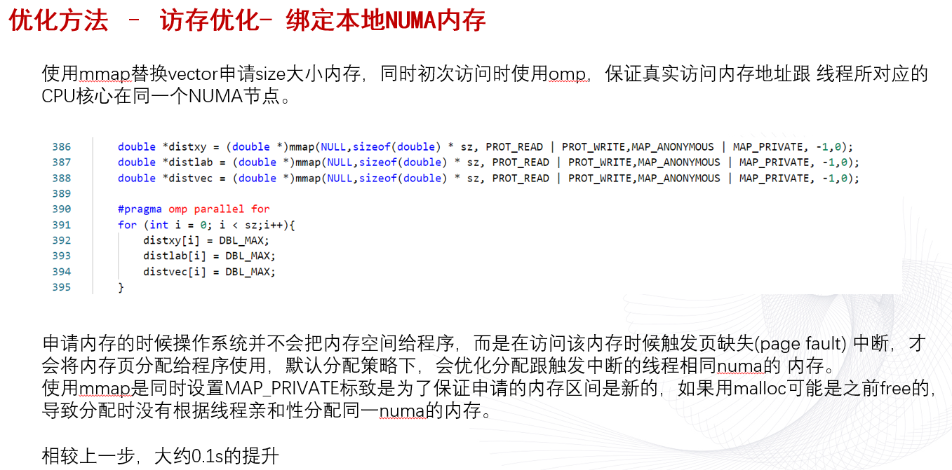
Vectorization
This metric represents the percentage of packed (vectorized) floating point operations. 0% means that the code is fully scalar. The metric does not take into account the actual vector length that was used by the code for vector instructions. So if the code is fully vectorized and uses a legacy instruction set that loaded only half a vector length, the Vectorization metric shows 100%.
1 | Vectorization: 23.7% of Packed FP Operations |
针对Vectorization: 23.7%的建议
A significant fraction of floating point arithmetic instructions are scalar. Use Intel Advisor to see possible reasons why the code was not vectorized.
SP FLOPs
The metric represents the percentage of single precision floating point operations from all operations executed by the applications. Use the metric for rough estimation of a SP FLOP fraction. If FMA vector instructions are used the metric may overcount.
X87 FLOPs
The metric represents the percentage of x87 floating point operations from all operations executed by the applications. Use the metric for rough estimation of an x87 fraction. If FMA vector instructions are used the metric may overcount.
X87是X86体系结构指令集的浮点相关子集。 它起源于8086指令的扩展,以可选的浮点协处理器的形式与相应的x86 cpus配合使用。 这些微芯片的名称在“ 87”中结尾。
FP Arith/Mem Rd Instr. Ratio
This metric represents the ratio between arithmetic floating point instructions and memory write instructions. A value less than 0.5 indicates unaligned data access for vector operations, which can negatively impact the performance of vector instruction execution.
小于0.5的值表示向量操作的未对齐数据访问,这可能会对矢量指令执行的性能产生负面影响。
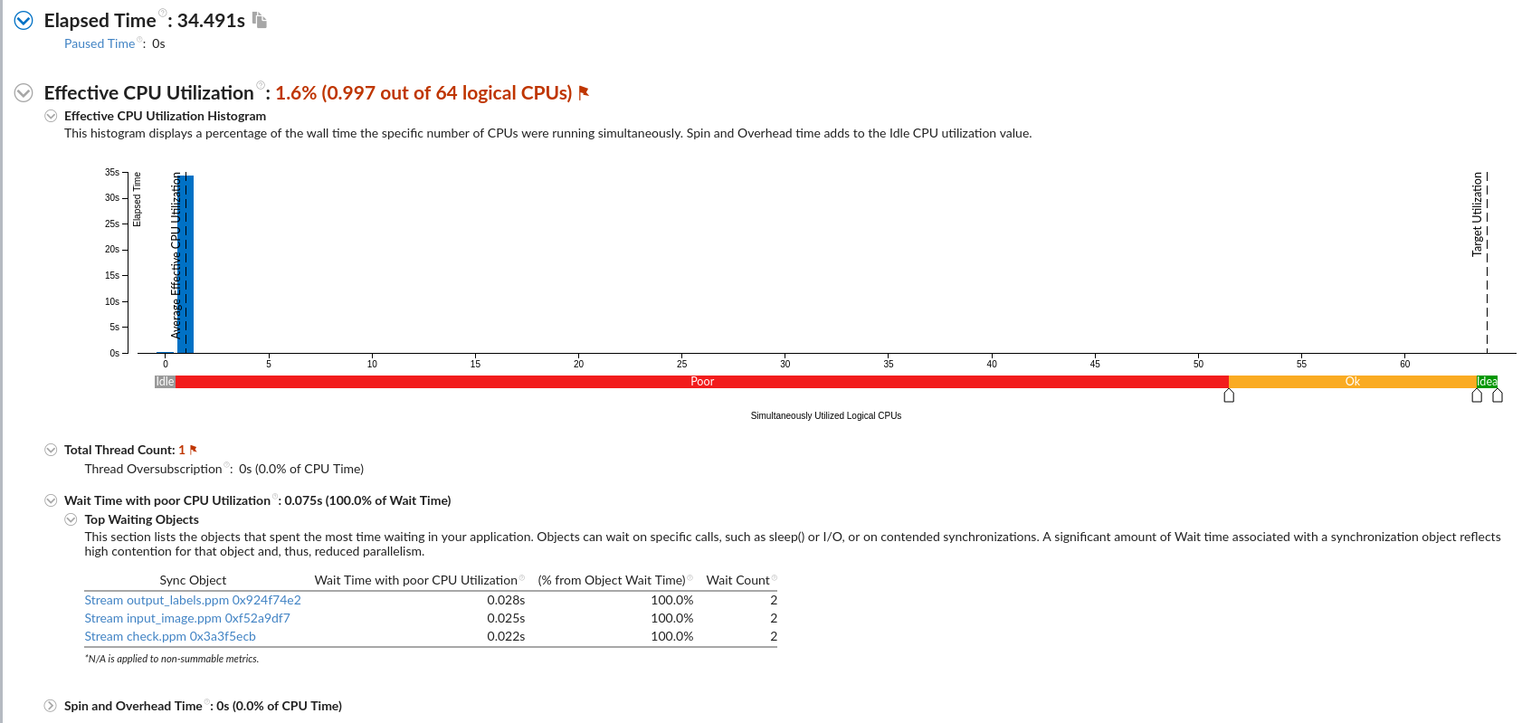
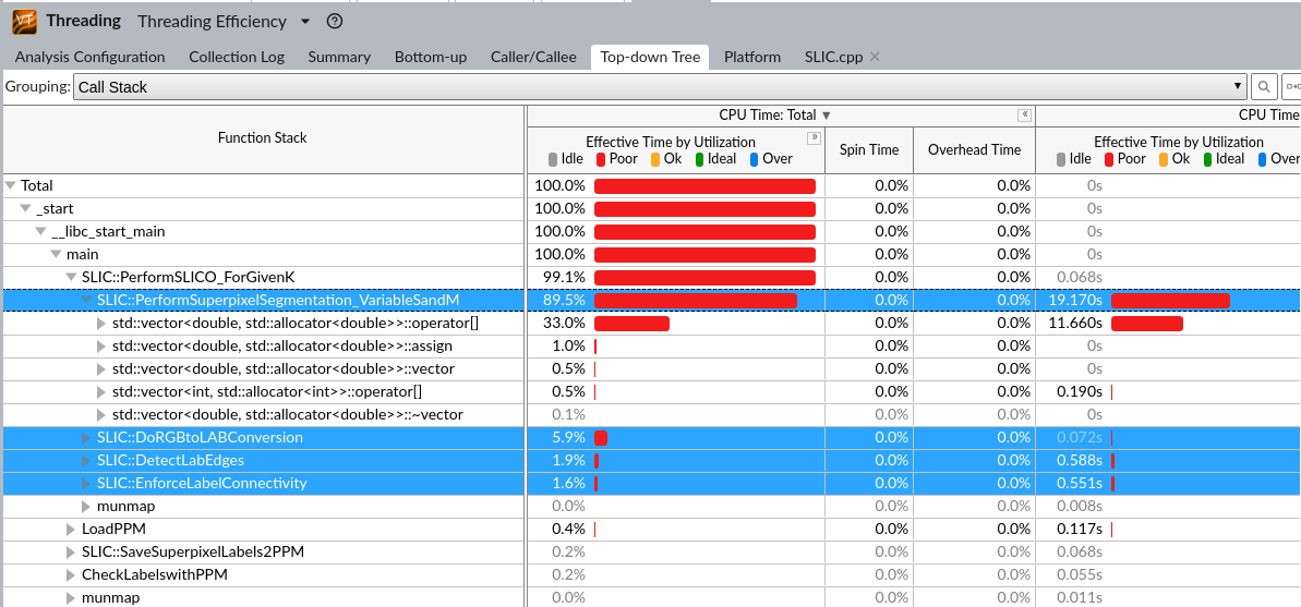
Step2 : Hotspots
User-Mode Sampling只能采集单核的数据,来分析算法的优化。
Hardware Event-Based Sampling硬件时间采集能采集全部核心,但是要少于几秒钟?
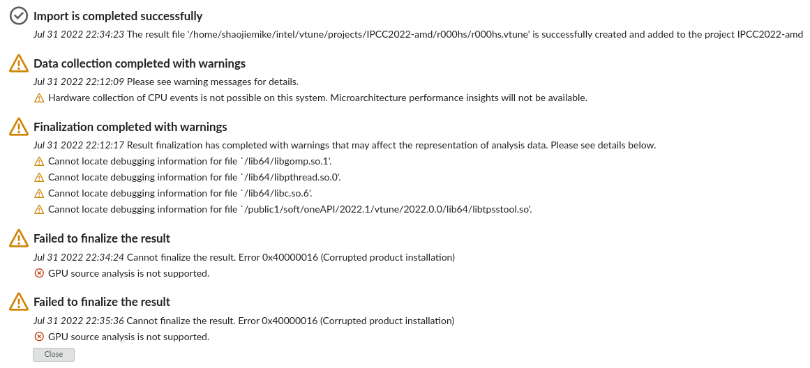
这个硬件采集慢,而且到一半报错了,发生什么事了?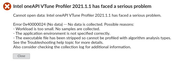

网上说是root权限的原因,但是我是用root运行的
反而用普通用户能正常跑Hardware Event-Based Sampling和微架构分析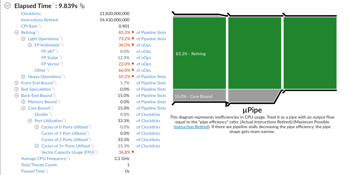
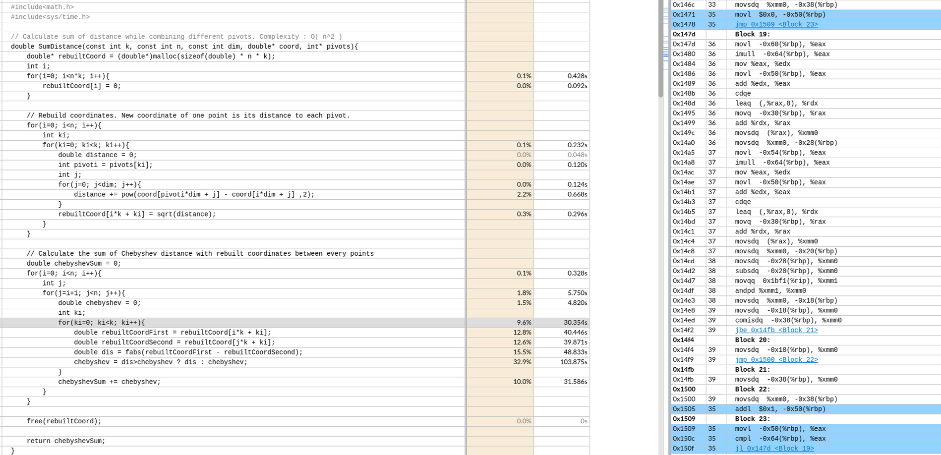
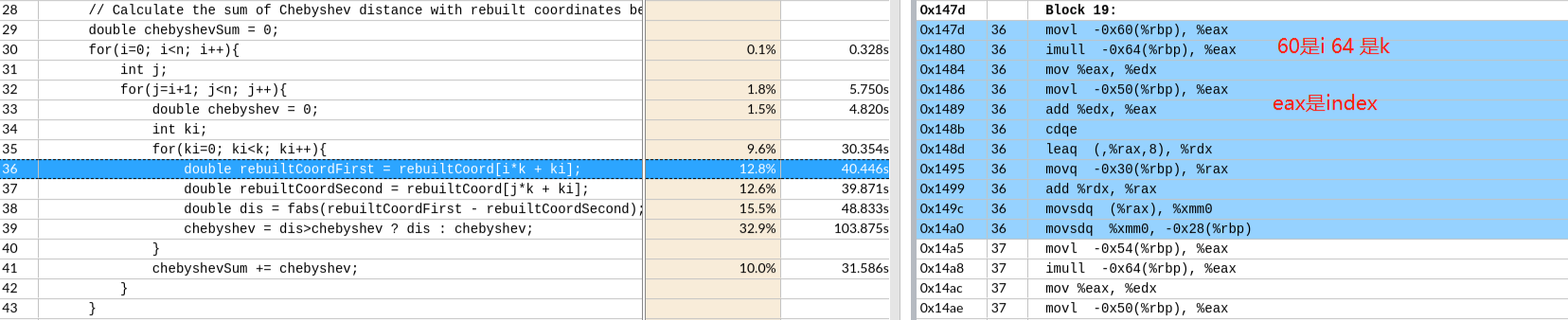
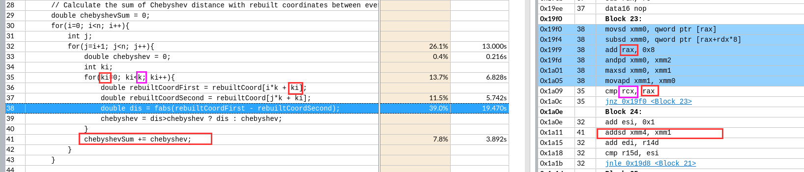
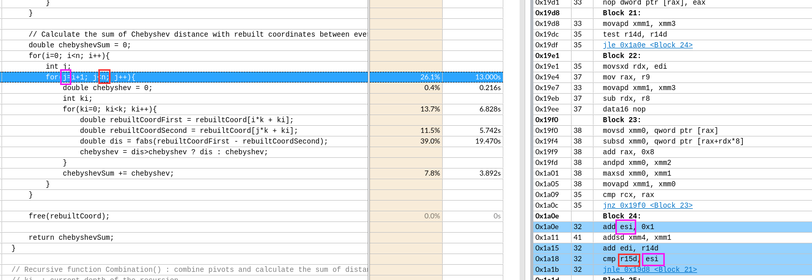
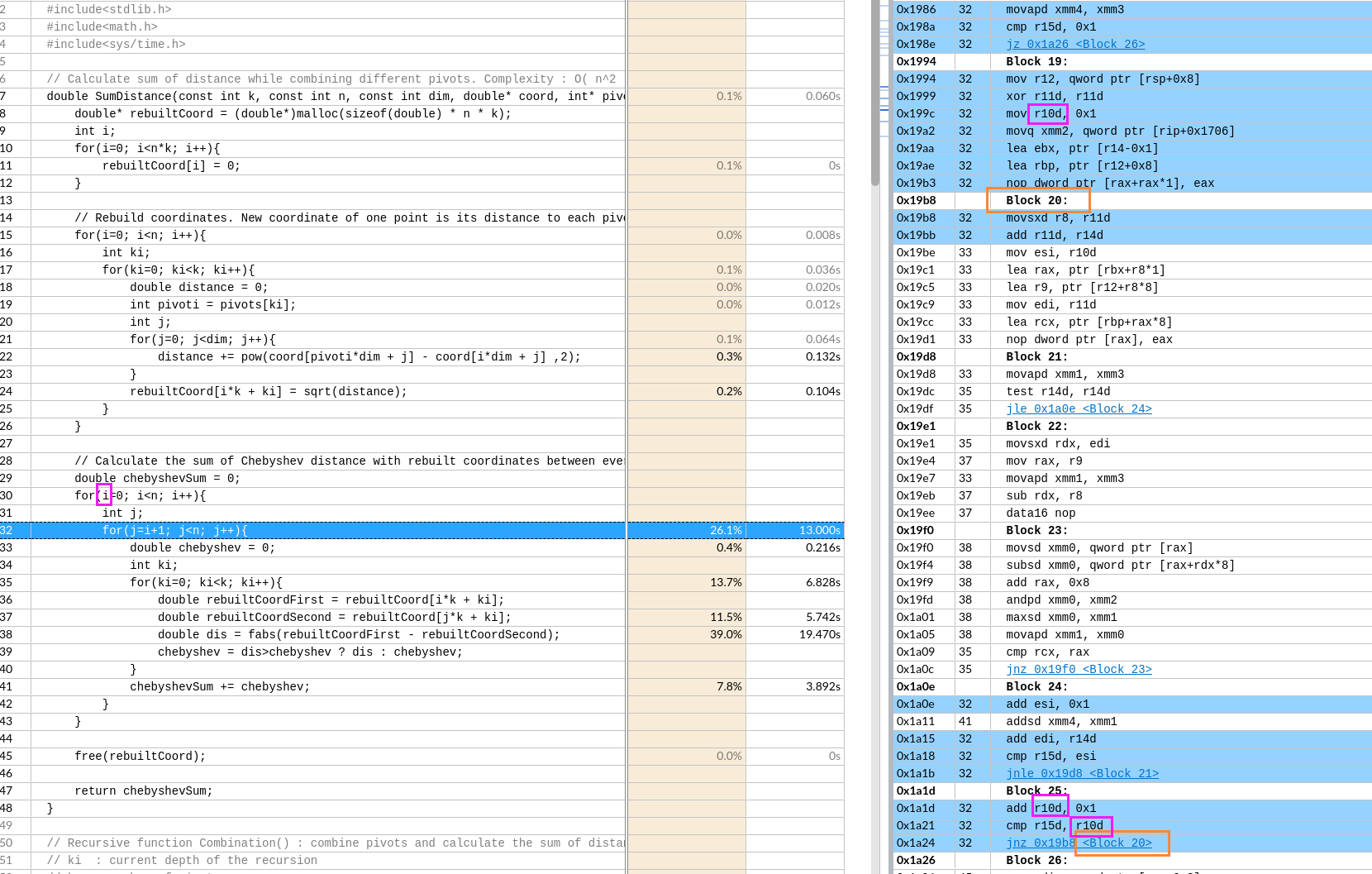
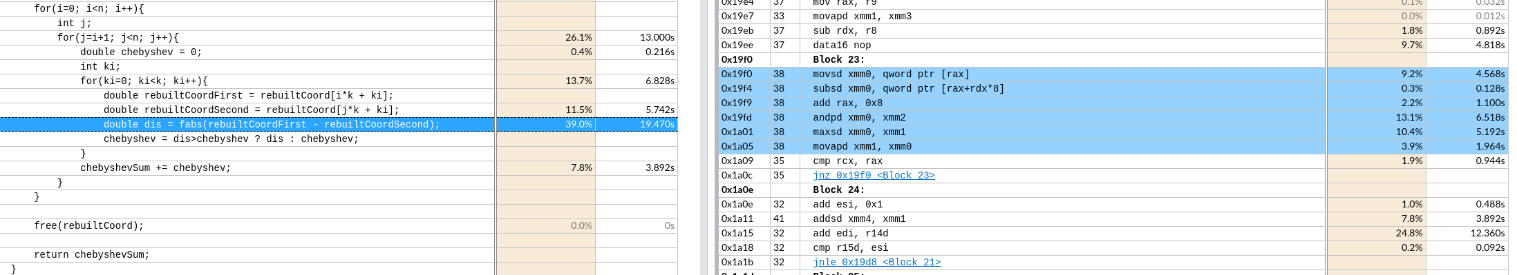
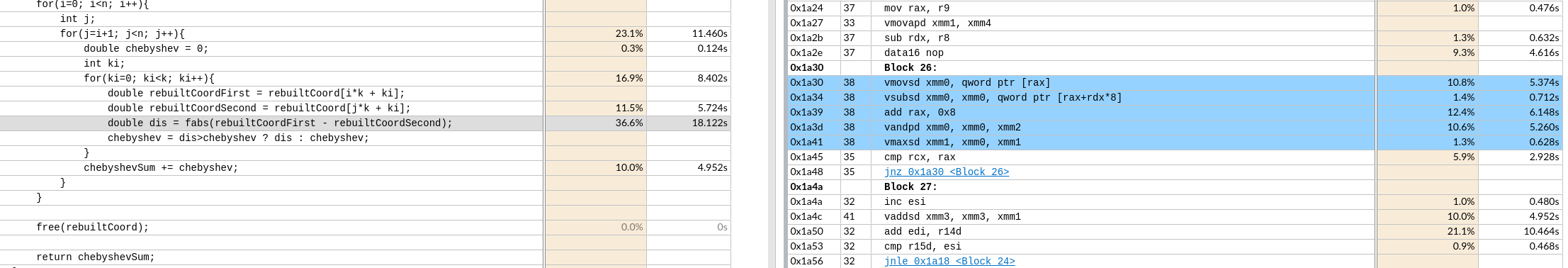
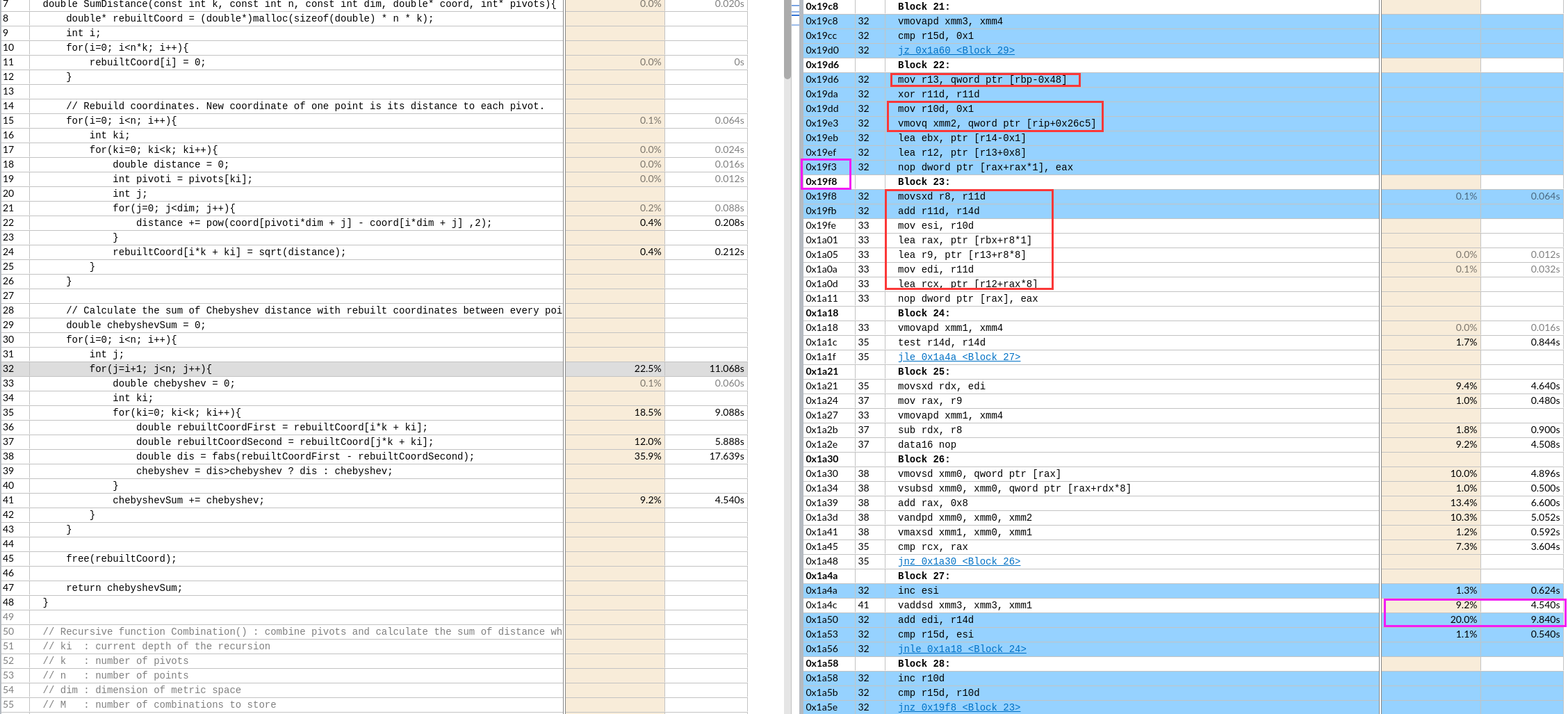
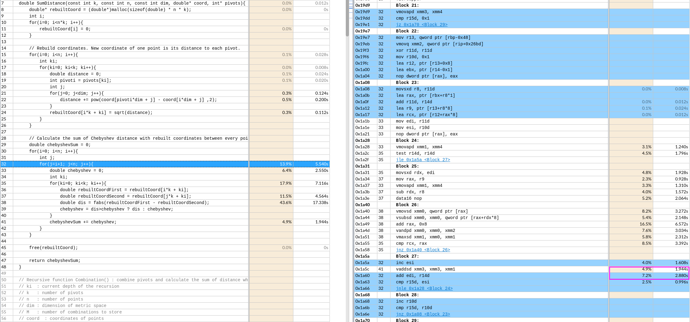
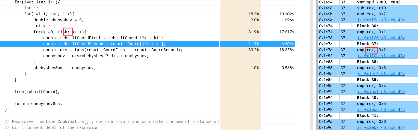
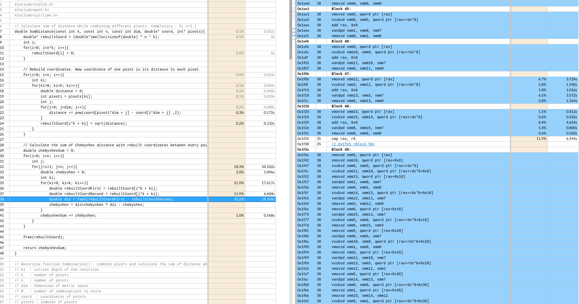
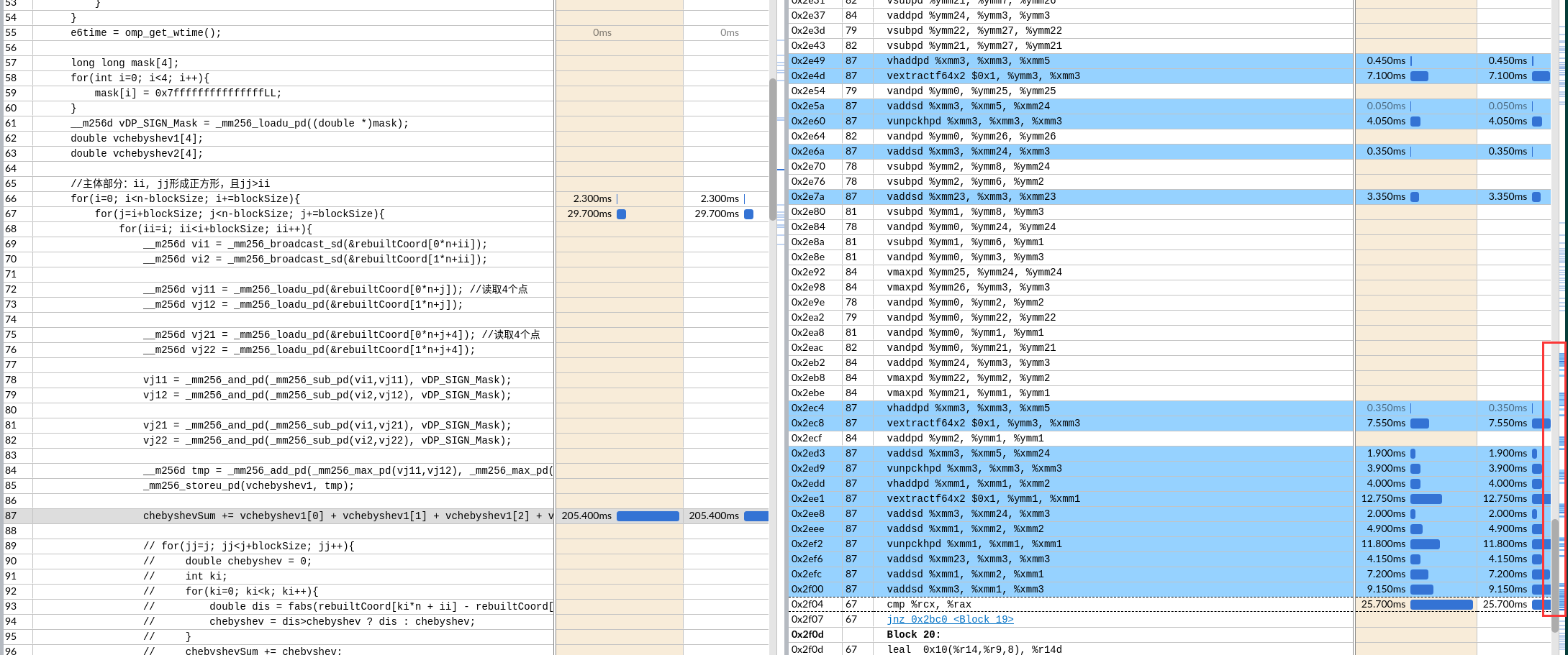
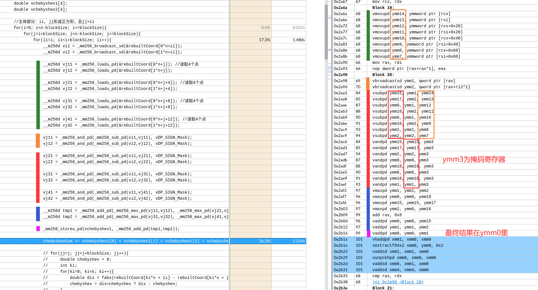
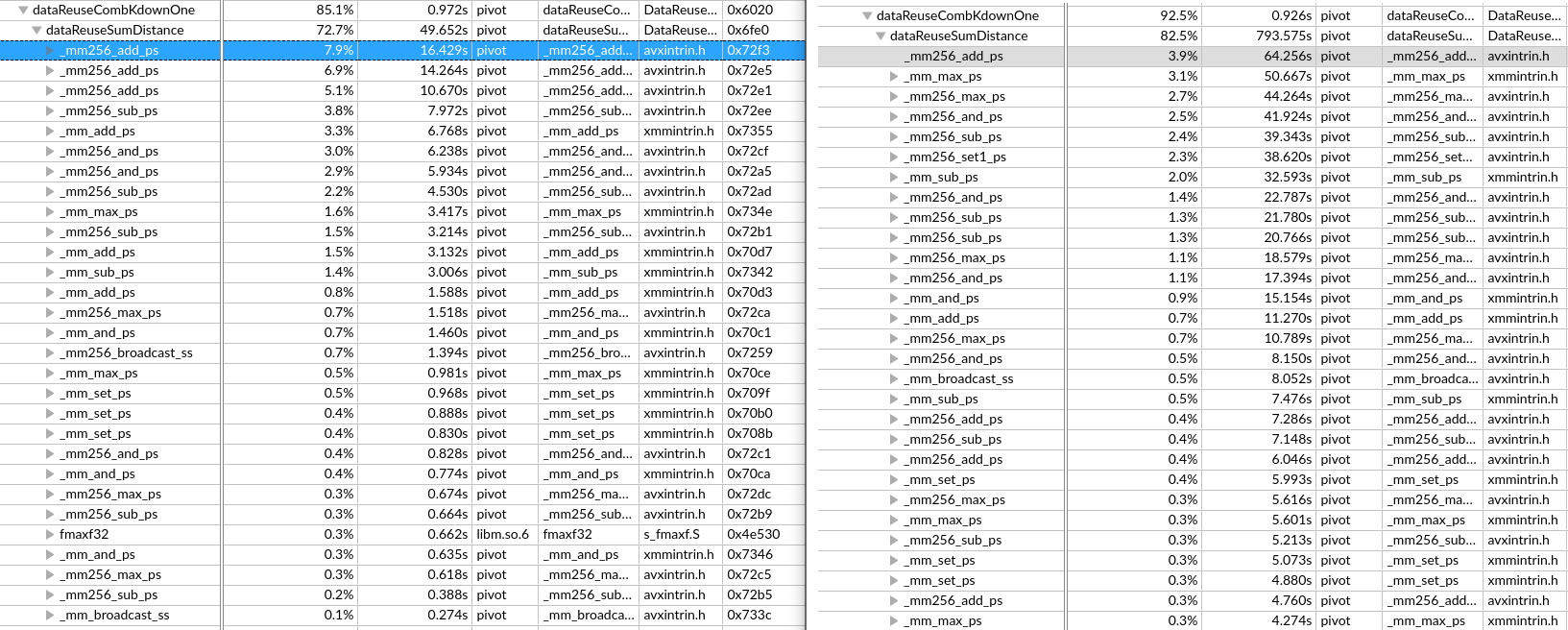
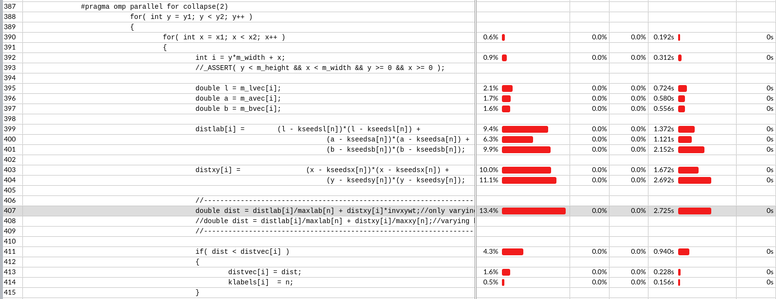
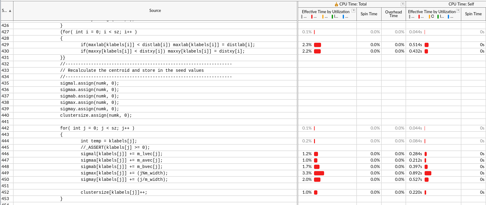
example
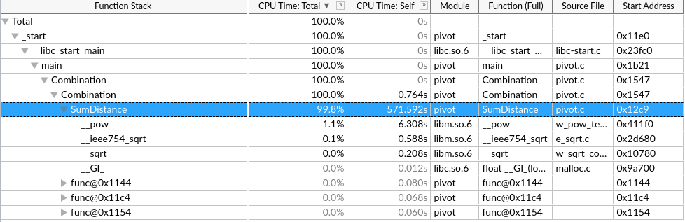
手动向量化该区域。
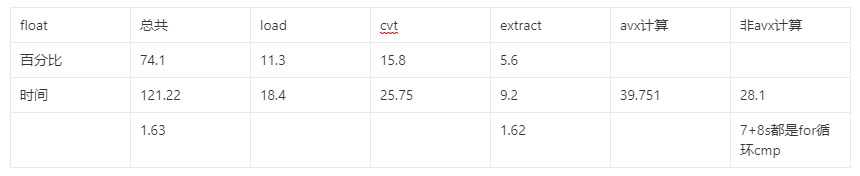
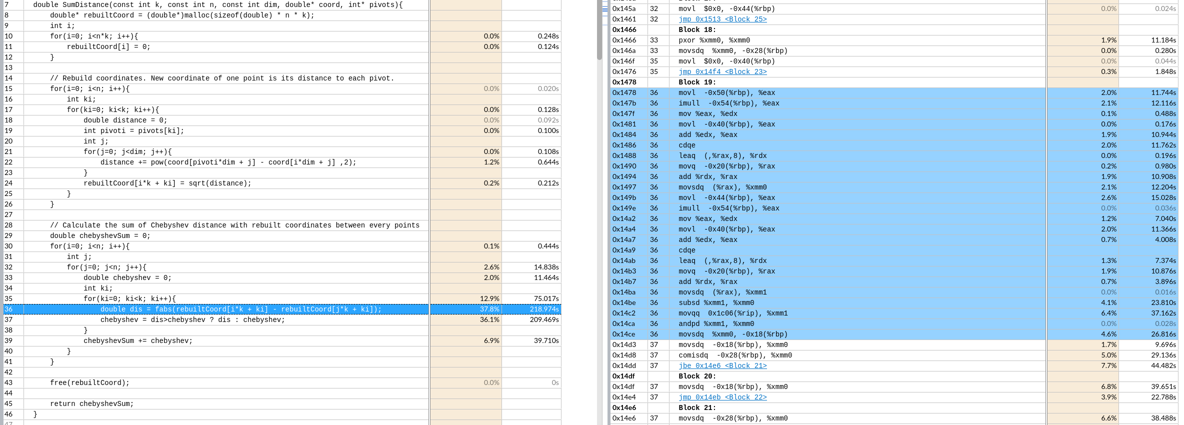
核心时间是 $k*n^2$ 次绝对值和,取最大值
优化思路:
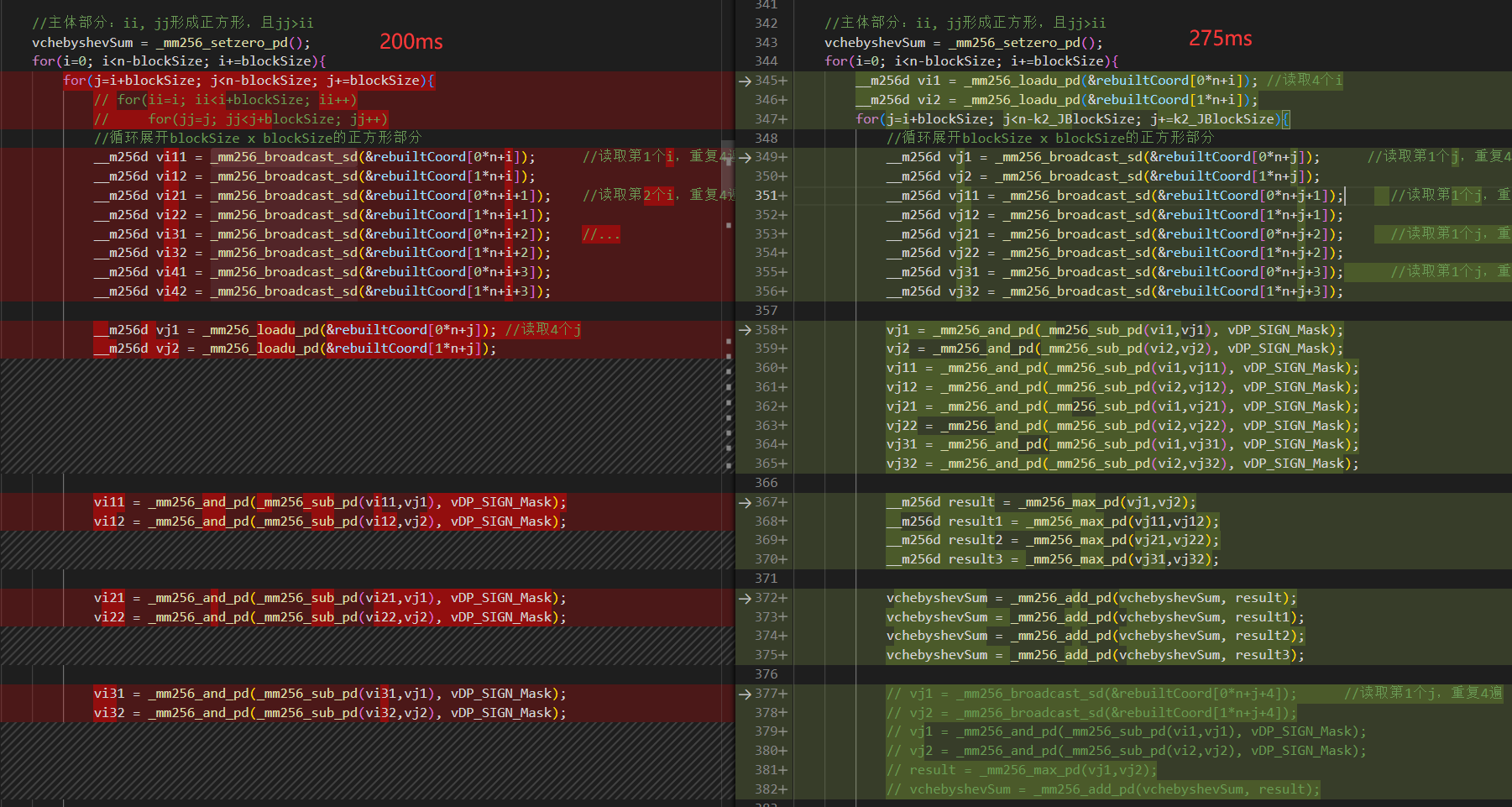
手动向量化(假设一次处理p个)
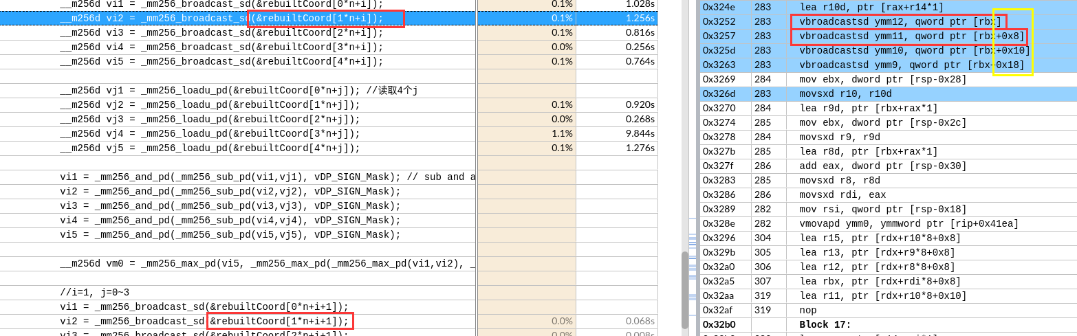
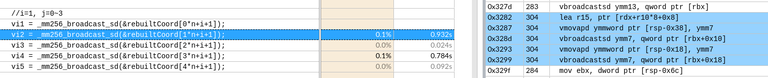
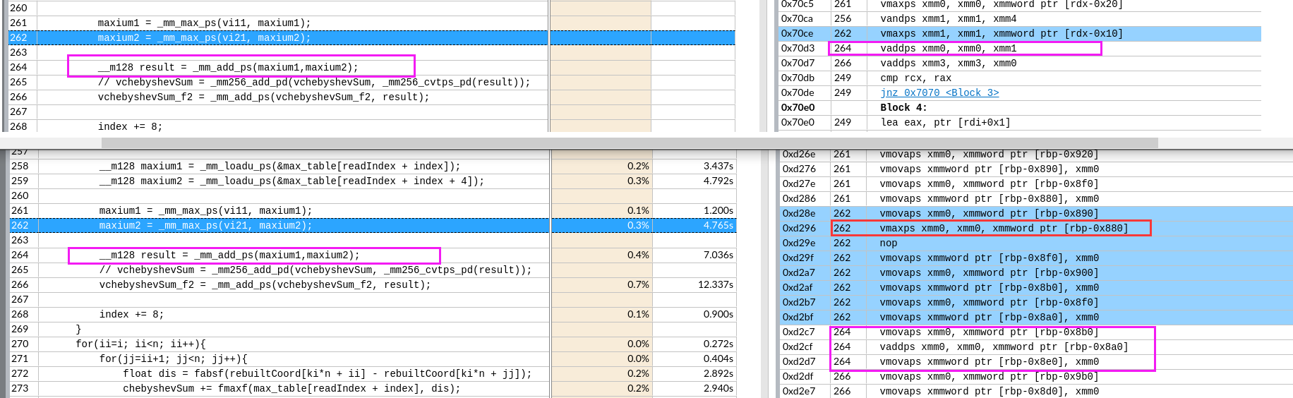
第一个n层取出 k个
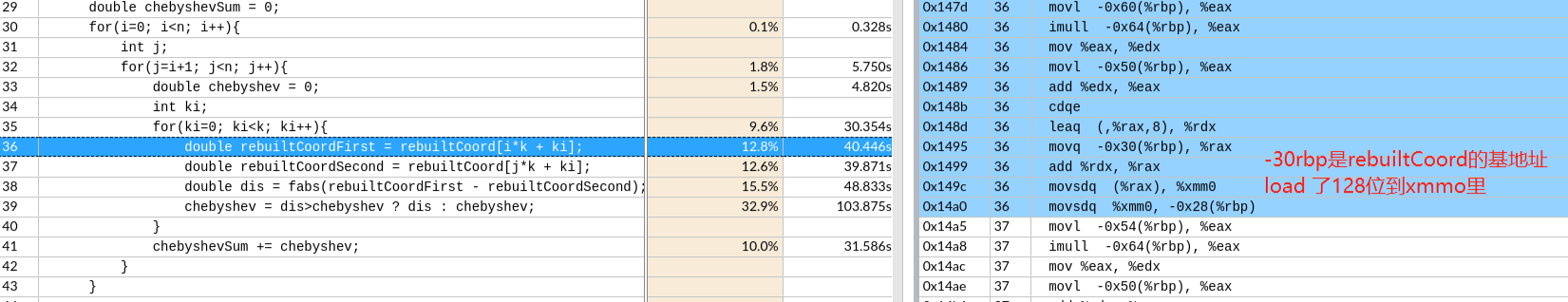
rebuilt[i*k+ki]重复读取到向量寄存器里,第二个n层取出k 个 连续的p个,到向量寄存器里。最后不足补0特殊处理,但是一般n都是4的倍数,可能可以不处理。8就要处理了。
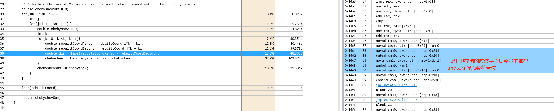
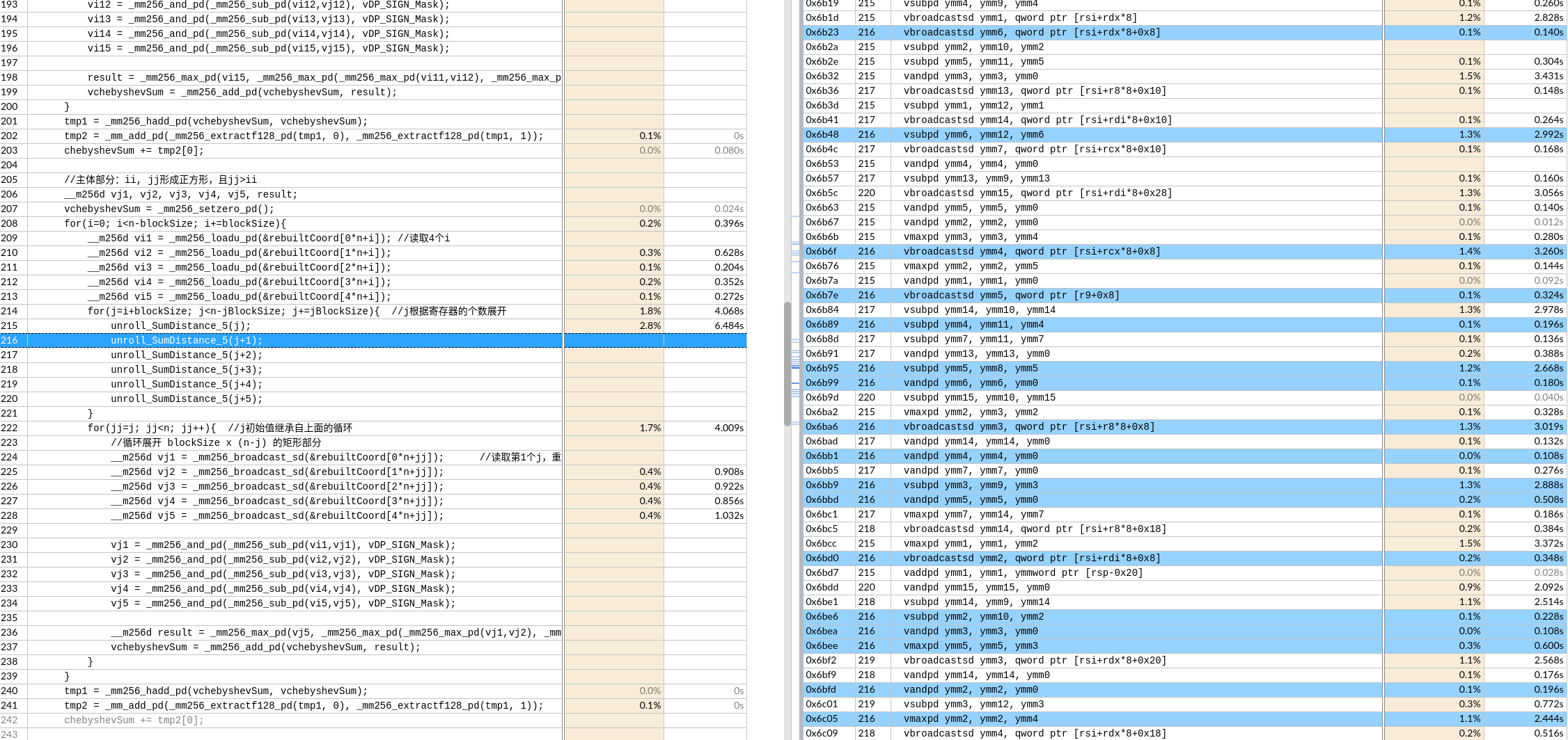
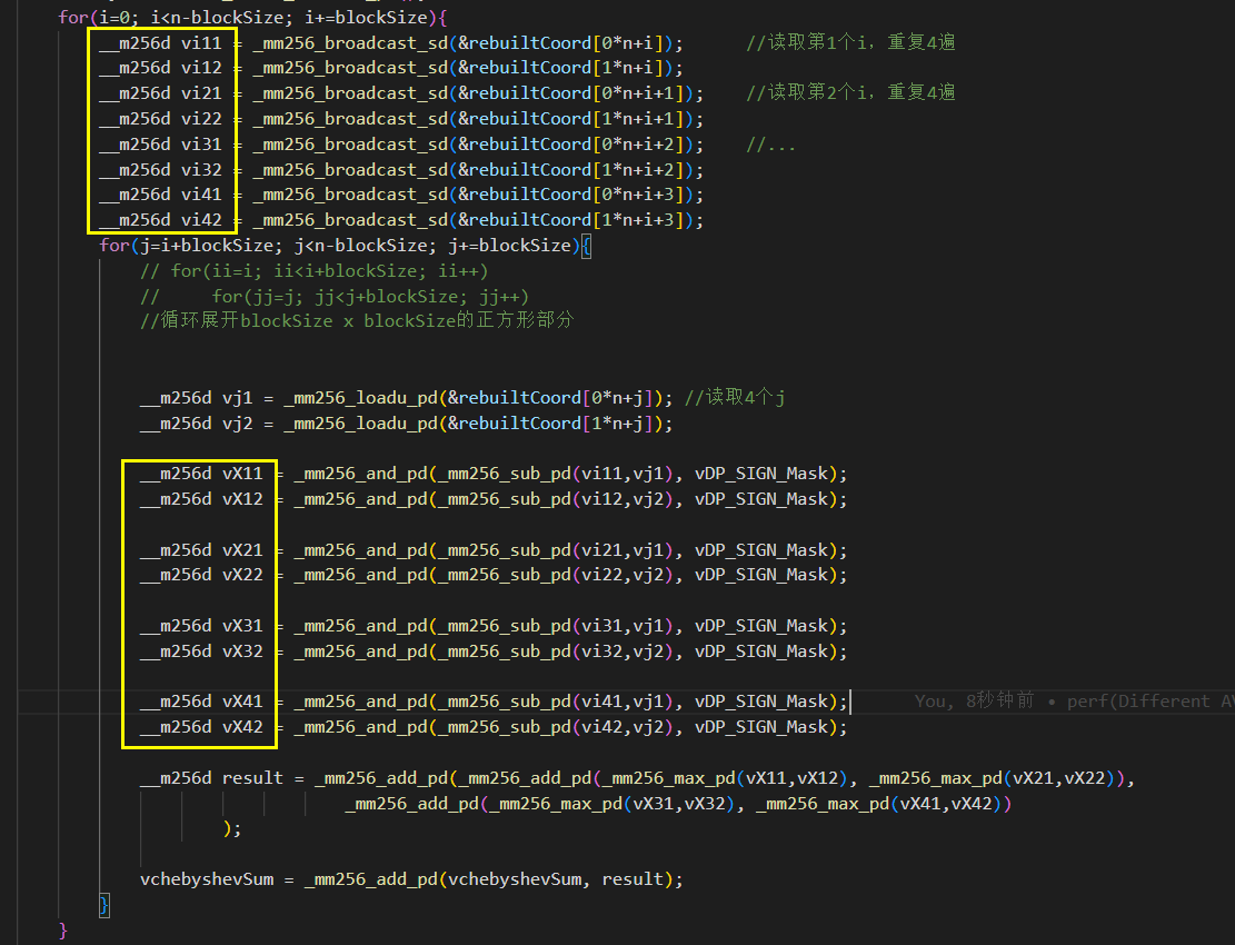
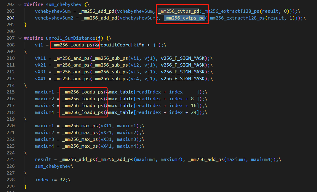
做向量fabs的结果缓存在k个向量寄存器里。
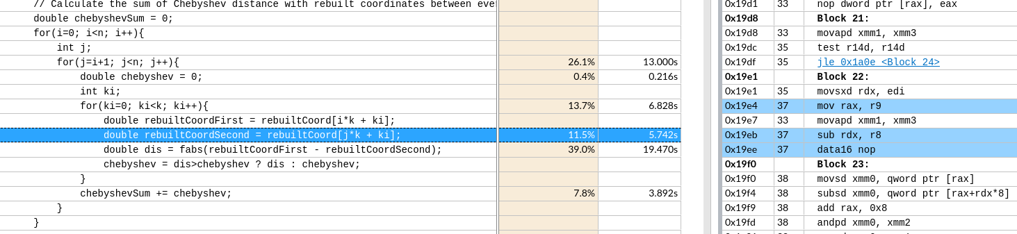
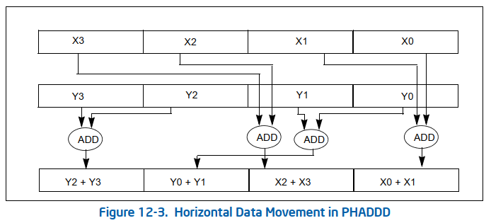
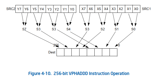
再对这个k个向量寄存器做横向的向量最大值操作到一个向量寄存器。不足的补0(取最大值不影响)
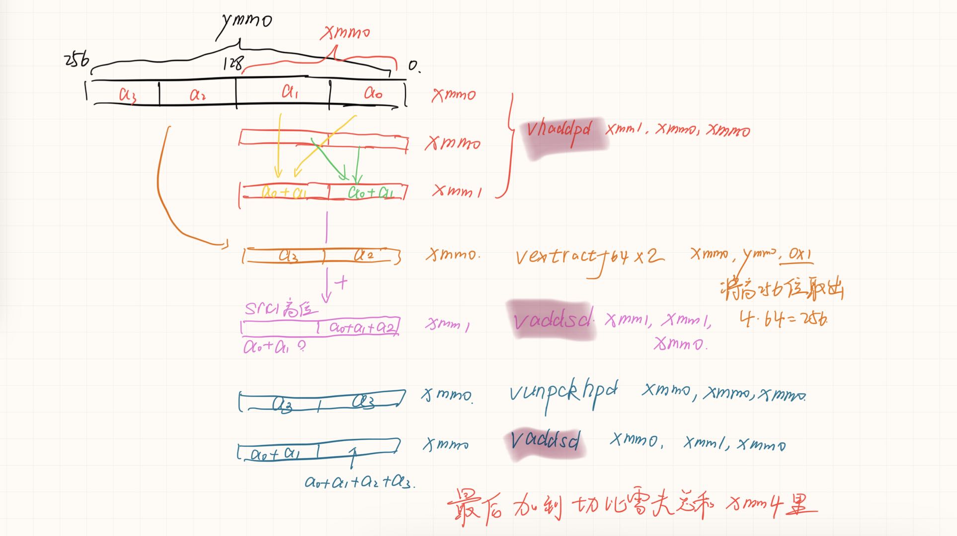
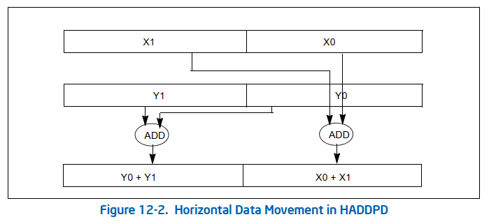
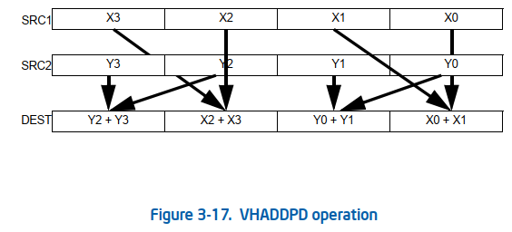
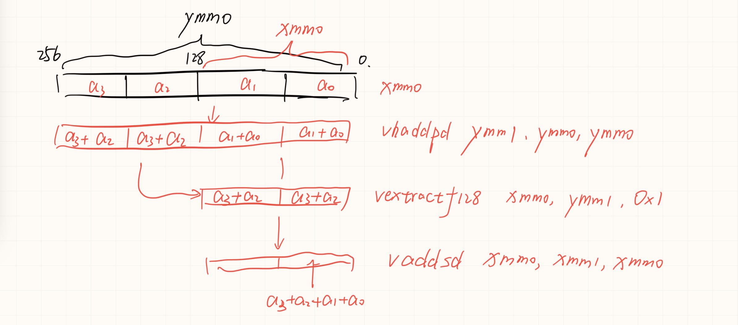
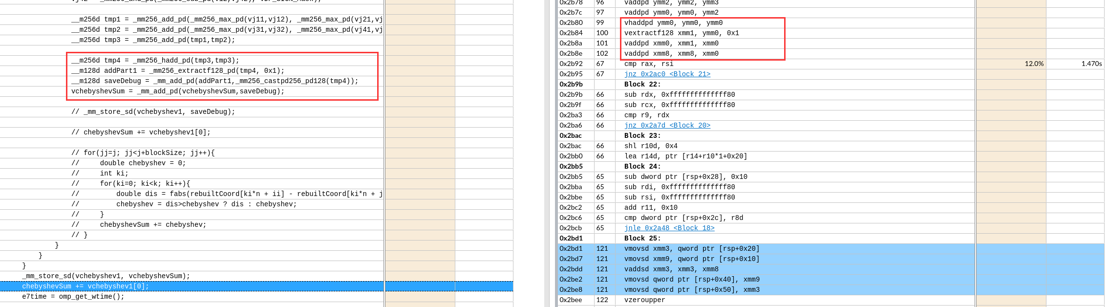
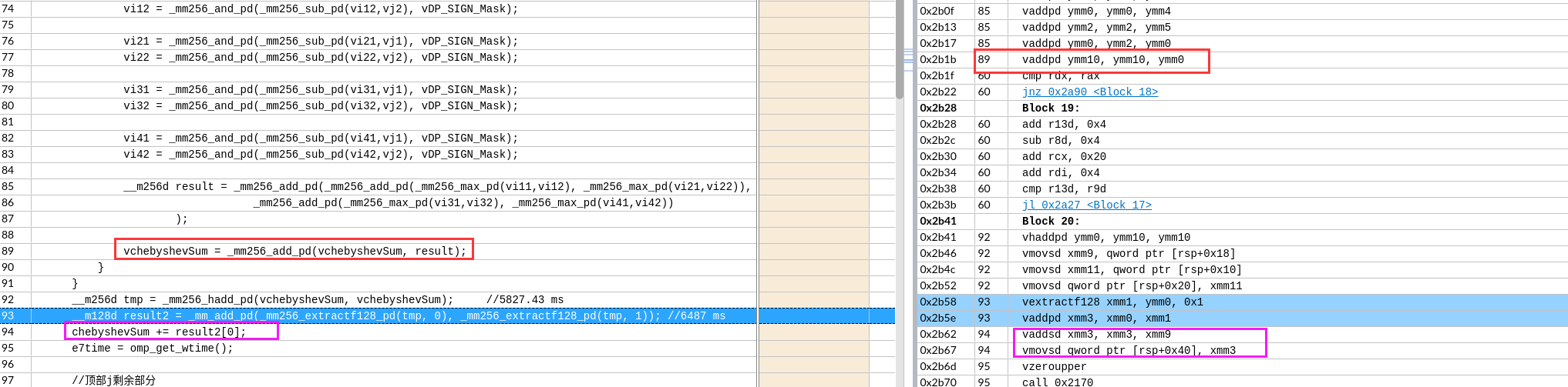
最后这一个向量寄存器做寄存器内求和,再加到
chebyshevSum里.这样就实现了p个元素的向量操作。这样一趟共需要3*k个向量寄存器。
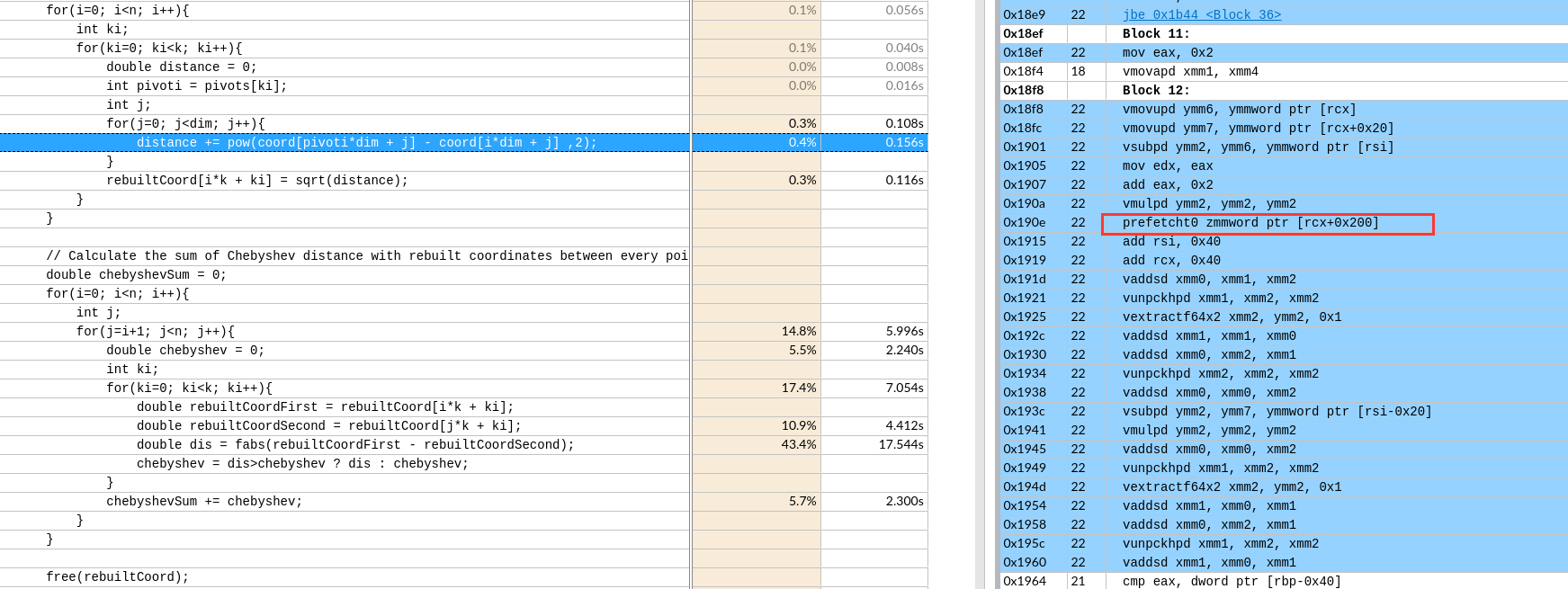
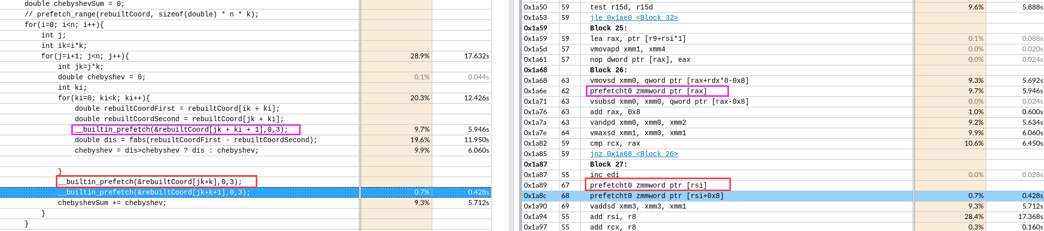
-
__builtin_prefetch()
手动循环展开形成计算访存流水
- 怎么根据输入来规模来展开?
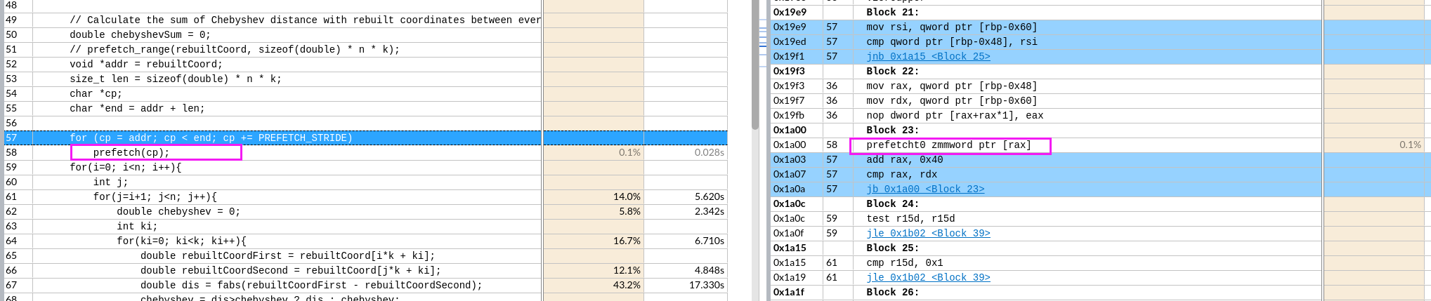
分块
访存分析
github对应项目与赛题
HPL-PL
复现机器
1 | $ lscpu |
baseline
1 | $ gcc --version |
优化步骤
由于O3和并行会导致热点代码不可读
在可迭代优化的例子下,根据vtune最大化单核性能。
很明显不是计算密集的应用,怎么形成流水最大化带宽利用,划分重复利用元素提高Cache命中率是重点(向量化对计算加速明显)
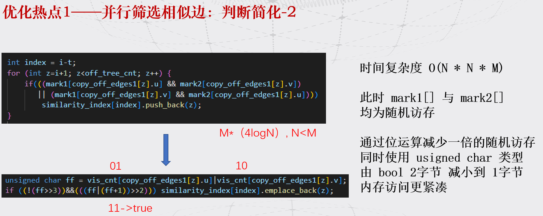
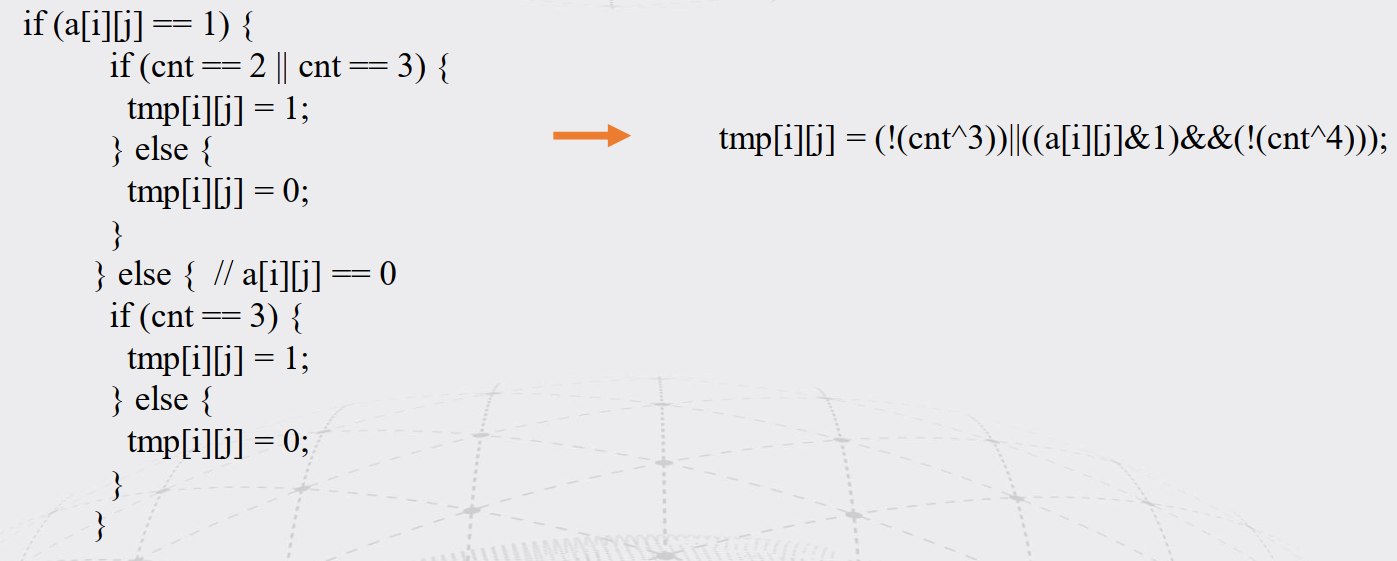
- 替换if
tmp[i][j] = (!(cnt^3))||((a[i][j]&1)&&(!(cnt^4))); - 去除中间不必要的拷贝
- int 变 char
- OMP_PROC_BIND=true 绑定线程到对应local处理器和对应local内存
需要进一步的研究学习
暂无
遇到的问题
暂无
开题缘由、总结、反思、吐槽~~
- 实验室同学黄业琦参加了HPC-PL全明星。想复现一下效果
- 之前Nvidia Nsight用得很爽, 想到vtune的访存优化部分和汇编对应的分析,使用的很少。想从提高计算流水和访存连续流水的角度结合vtune优化。